

Pipe 7: The e,f,g,h, and kw pipeline
Pipe 7: The e,f,g,h, and kw pipeline
The e-pipe for short.

A half-pipe to get started
The SHA-256 “digest” takes 256 bytes and mixes them around within a stage. There are 64 stages, all doing the same mixing. The mixing is designed to randomize the outputs but it also uses only functions that deliver 50% chance of 1 or 0 on their outputs, keeping the overall function balanced. The stage is defined to operate on eight 32-bit words, named “a” through “h”, plus a word of 32 bits from the data which a separate “scheduler” function (not shown) mixes in a different and slightly simpler way before passing to the digest.
The diagrams carry a lot of detail, I do recommend you view this on a large screen if you can. On a mobile you can view sideways, or tap the images to load them in the browser where you can zoom. I use subsets of the design where I can, but at this point the wires flow across multiple library cells and smaller views do not allow you to see where things start and finish.
Reducing it to 32 separate slices
The 32-bit words are rearranged as 32 columns, or “slices” or “pipes”, each of which process bits {a,b,c,,e,f,g,kw} where “kw” is a bit from the scheduled data words “w” combined with a pseudo-random constant “k”. These 9-bit slices mostly connect internally, just getting or giving come carry-bits to their neighbors. All 32 slices are the same, so out design problem begins with optimizing this repeated building block.

The diagram below shows how the bits flow through the slice. The slice is split into halves with bits {d,e,f,g,h,kw} placed first (called the e-pipe, which ends with a new “e”) then {a,b,c} forming the second half (called the a-pipe, which ends with a new “a”). This order, e before a, is partly because kw is ready early from the scheduler, but mostly because some of the e-pipe internals are needed as inputs to the a-pipe.
The {e,f,g} bits are passed to the next stage in place of {f,g,h} with the original h discarded, while the {a,b,c} bits become {d,e,f} in the next stage.

The blue boxes to the left of each half-pipe are fed e-bits or a-bits rotated from other slices of the previous stage and mixed in a 3-bit XOR. The rotation will be done with a set of 32 wires for each, e and a, that spread across the whole stage and do not have any “rotation” logic in the column - just connections to the correct wires.
The kw bits are also delivered by a set of 32 overpassing wires. We will add the rotation and kw wires to the model after the logic. The layout will need to ensure there is space for those sideways, upper wires to be connected to the inputs in the logic. We will also need output buffers (amplifiers) after the e and a results of a stage, to drive those rotation wires.
Stages start with latches
The stage inputs are all latched is so that the pipeline works correctly. Every SHA-256 function uses 64 stages. At any one clock the value is only in one of the stages, it hasn't reached the next stage yet and the entry latches to the next stage are closed.
The data values move from stage to stage when the latches are enabled by a brief clock pulse. When the values come out of the last stage the calculation is complete. The other 63 stages are always working on different values. The magic of pipelining is it separates the overall function into small stages which can be cleanly designed and finish on a fast clock, while all the stages work at the same time but on a different calculation keeping everything busy. The pipeline delivers a new completed function out of the final stage on every clock. The two SHA-256 pipelines joined together to total 128 stages overall so actually the blockchain calculation is running 128 calculations on every clock cycle. Each stage is simple so the clock can run fast, and then that's clock rate is multiplied by a 128 to give us the very high rate of calculation we want.
This post will describe the e-pipe, and the next post will describe the a-pipe, the connection between them, and the side-by-side layout of multiple pipes to make a stage. A third post will discuss issues around carry look-ahead, buffering, clocking, and power distribution. In a fourth post this is all joined together in two SHA-256 pipes with 64 stages each and some control logic at the beginning and end.
I welcome discussion of the open section of the post, you can add comments to the Table of Contents for Pipeline post if SubStack will not allow your comments here. Thanks!
Thank you for supporting this blog.
The e-pipe in detail
The e-pipe handles the d, e, f, g, and h bits of the digest, mixes in a kw bit from the scheduler, and calculates a new e bit. It is the first part of the digest slice.
A dual rail configuration is chosen. Two rails is enough to allow all the wiring to fit cleanly into the lower metal layers. The length, 7.4 microns, is going to be enough for us to fit the 3 groups of wires that pass overhead for the kw signals and for the e and a rotations. 96 wires overall using the 60nm pitch of the M5 layer available in the model for 4nm process assumed for this exercise would be about 6 microns, so if we used more rails and a shorter slice it would cause routing problems.
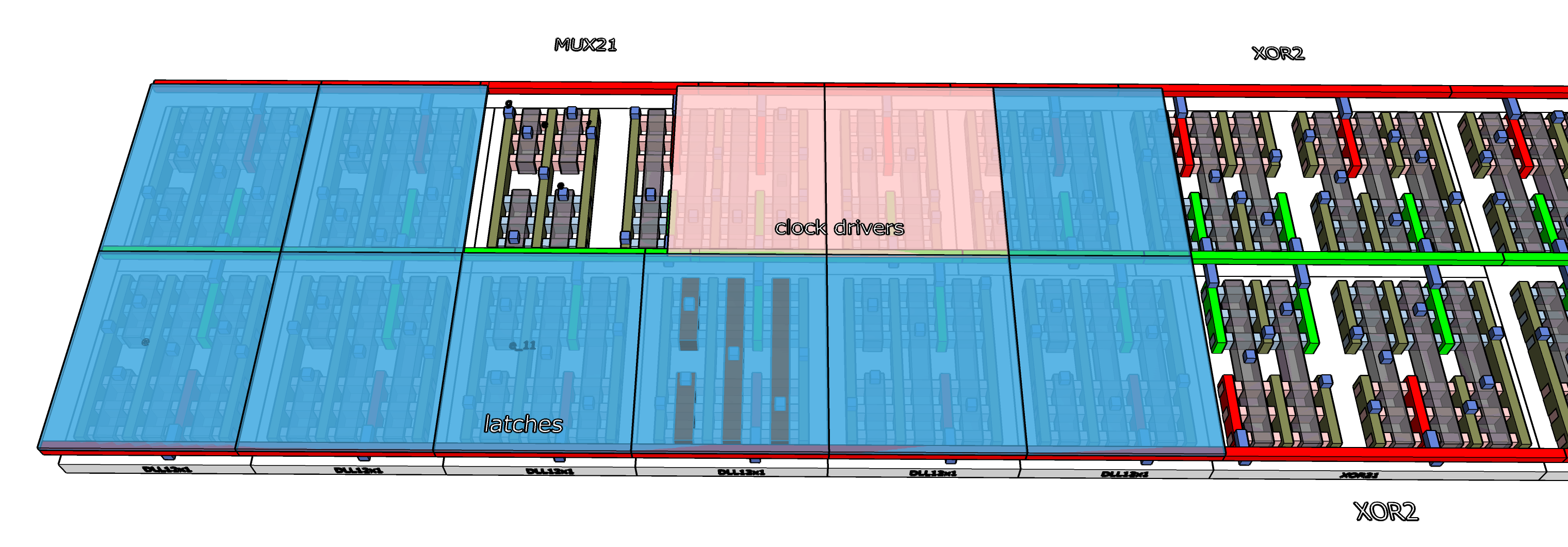
The standard library cells are mirrored when used in the lower rail, where Vss is now at the far side. Three other cells are mirrored horizontally. The first is the MUX cell which is 3rd from the left in the far rail: this was done to allow its powered edge to merge with the clock drivers. The XOR2 cells towards the center, one in each rail, are mirrored to place inputs closer to the left and output closer to the right. I would expect these tricks are used by EDA tools when they do automated layout, too.
Each stage starts by latching all the inputs as close as possible to the same moment in time, controlled by the clock pulse which is narrow enough to take a sample but not long enough to allow new calculations to arrive. The e-pipe and the a-pipe can clock their latches at slightly different times, as long as the groups of inputs to each half pipe are grouped on the same clock. The a-pipe is going to be dependent on some outputs from the middle of the e-pipe so we can drive the a-pipe off a slightly later copy of the clock.

The clock, which comes in from a sideways wire connected to a single load, seen reaching up at the far right, which is amplified in three stages to generate the CLK and ~CLK signals distributed to the 9 input latches. Everything has been kept close to keep the input signals as simultaneous as possible. The buffers have been connected by double-vias and double wires to improve delivery from the gates to the signal wires on metal-0. Those signal wires are less than a micron long which should deliver the signals in less than a picosecond, much less than the rise time of the transistors in the latches. We will come back to further optimizations in a later post.
Routing the latches to logic cells
The outputs of the e-, f-, and g-latches feed into the MUX logic cell which is 3rd from the top left and creates the “Ch” value inside the slice. These connections are solved with local M0 and M1 wiring. There are also 3 rotated e-bits from other slices which will come in from overhead wires. Those latches, for rotations of 6, 11, and 25, are set side by side on the lower rail and their outputs feed into the two XOR2s which together form the XOR3 which creates the Σ1 value.

The other 3 input latches are for the d, h, and kw inputs, which will be routed into the adders further to the right.

The M2 layer is used for these longer connections, along with the inputs from the prior stage, entering from left, and the simple repeated outputs f_out, g_out, and h_out which are driven to the right starting from the outputs of the e, f, and g latches. There are some other places the M2 layer was needed to solve local wire crowding.
This crowding would be harder to solve if the track height (actually width on the chip, but it is called height since that is how illustrations are drawn) shrinks. If track height shrinks but backside power delivery is used, where power wires move to the back instead of taking space on the front, then the available local wiring in M0 and M2 should remain about the same. That should be a nice process change.
The full adders
A full adder takes two input values, locally named A and B, and adds them together with a carry bit, named C. Strictly speaking all 3 bits are equivalent so we could connect whichever source is easiest to layout for each of the A, B, and C inputs but in practice the path from carry-in to carry-out should be faster than the other inputs, since carry propagation is usually the main delay in adding multi-bit numbers. In the M1 layer you can see the carry paths in the 2nd, 3rd, and 4th adders come in from the top side and exit from the bottom side, while the A and B inputs are found to the left.

When we add in the M2 layer we can see that the connections for carry ripple are kept short, but the wiring resources keep the A and B on fairly short connections too.

The two-rail design allows for compact wiring. M1 going sideways handles a lot of signals.
This layout, as with others in the blog, has not been verified. It is an exploration for study, not a product ready to be made. The rules used are cautious, but there may be some choices that do not work as expected.
Mind the gap
I have left a gap at the end of the e-pipe. The a-pipe will begin to the right of the gap. This allows for wiring swaps with the M4 level, but will also be used later for carry look-ahead and for buffering the “e” output as it connects to the rotation wires.
The look-ahead and the rotations will make more sense when we have multiple slices to look at, so I will come back to those functions later.
The wiring changes move some of the e-pipe outputs up to M4. They will pass over top of the a-pipe and come back down for use in the next stage of e-pipe. You can also now see that signals a, b, and c have been on M4 passing overhead of the e-pipe, and these will be brought down to be inputs to the a-pipe coming up next, on the right side of the gap.
You can also see the eCarry1 line in the gap. It is the only carry which flows both between slices but also from the e-pipe to the a-pipe, so the gap is a good place to route it.
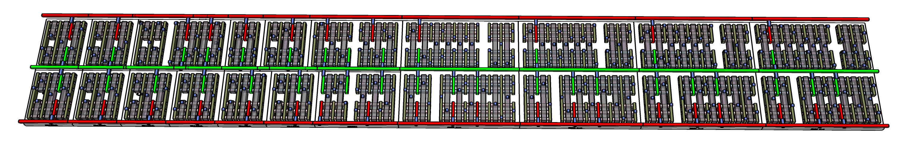
Let’s see that again
As a video.
That’s a wrap on the e-pipe.
Next week
Next week will be about the a-pipe which forms the second half of the slice, connecting it to the e-pipe and other signals, and then group multiple slices together to show how all the sideways signals flow.